In a previous post, I implemented a linear regression model that created a prediction for the total number of wins a team would achieve in a single season.
To continue learning about predictive models, I built a logistic regression model to predict in-game win probability.
How likely is the current team to win the game given the current score, position on the field, yards to go for a first down, and other attributes?
The play by play data comes from the nflfastR package for R (using the 2009-2020 seasons). See the GitHub repo for my source code for this project.
3,184
Games
14,697
Scoring Plays
473,356
Total Plays
In the chart below, the black line is my model; the grey line is the built-in nflfastR prediction model. The solid marks at the top and bottom of the chart are scoring plays. The home team’s logo is displayed at the top and the visiting team’s logo at the bottom.
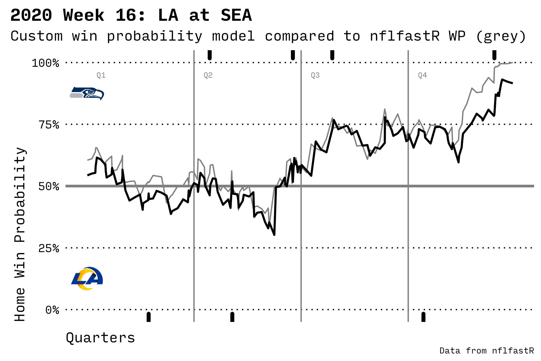
An exciting game where Seattle beat LA in the 2nd half
It’s interesting to observe how the probability of winning rises before a scoring play. The model knows that, as a team approaches the goal line, it’s more likely to score. Then the probability of winning drops away after a score since the other team has the ball and is gradually increasing their probability of scoring.
It’s also fascinating how the data shows a slight advantage for the home team even before the game starts. This wasn’t specifically programmed into the model; the advantage just appears based on some attributes and the final game outcomes.
What does win percentage mean?
A common misunderstanding is that any win percentage under 50% means that a team will definitely lose. This is incorrect…anyone can win, even with a 1% chance of victory.
Here’s how it works. A 10% win percentage for team A means that if this exact game were played ten times, then team A would win one of those times.
The other misunderstanding is that win percentage is somehow omniscient and factors in any injuries, bad bounces, or lucky catches that might occur later in a game. It doesn’t! A 10% win probability for team A means that given what we know right now, if these teams continue to play in the same way that they are currently playing, then team A will win 1 out of 10 times. If anything out of the ordinary happens, then the win probability will change.
It does include an average injury rate and an average lucky catch rate over the 3,000 games in the dataset. But if a team has a greater than average number of injuries (or to an irreplaceable player like the quarterback), then the outcome may diverge from the prediction.
The Model
A logistic regression model predicts a result in the range of 0 to 100% which works well for a sporting event where one or the other team will win. My model uses nine attributes that change throughout the game. I generate a new prediction after every play. The attributes used are:
| Attribute | Description |
|---|---|
qtr |
The quarter: 1, 2, 3, or 4 (overtime is ignored) |
down |
The current down: 1, 2, 3, or 4 |
ydstogo |
Number of yards left to gain for a first down |
game_seconds_remaining |
Seconds remaining until the end of regulation |
yardline_100 |
The line of scrimmage on the field (where the ball is placed) |
score_differential |
Number of points ahead (plus) or behind (minus) for the current team |
defteam_timeouts_remaining |
Unused timeouts for the team currently on defense |
posteam_timeouts_remaining |
Unused timeouts for the offense |
is_home_team |
1 if the team in possession of the ball is the home team, 0 otherwise |
As is often the case with a data prediction or reporting project, most of the initial work was about finding my way around the available data and figuring out what columns I needed in order to calculate others. The nflfastR dataset includes over 300 columns per play, and there was no authoritative field reference until after I completed the majority of the project (there is now a useful page with field descriptions).
Some fields have null values which must be ignored or filtered out, and other useful columns must be built from a logical combination of other fields and values (such as determining whether or not a play constituted a scoring play for the home team).
Once I had all the columns in place, it seemed like magic to send it through the glm() function in R and receive a predictive model back. There’s no need to calculate how many plays occurred at each position on the field or group events by a specific time in the game. You just send over all the columns you care about, tell it what field represents the positive outcome (winning the game), and it does all the rest.
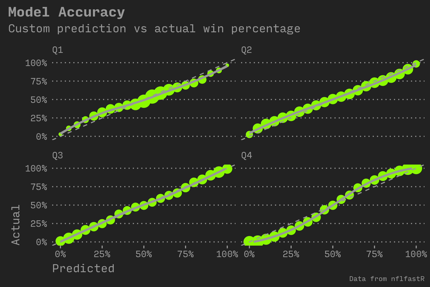
A standard way to gauge the accuracy of a predictive model is to compare the estimated win percentage to the actual. I followed the example from a blog post describing the built-in nflfastR model and split out the estimate by game quarter. A straight line of green circles indicates an accurate prediction. If a circle is further away from the dotted reference line, it indicates that the model predicts incorrectly for that percentage range. I also rounded to the nearest 5%.
The dot size shows the number of plays in the sample set. The 1st quarter has very few samples for teams with less than a 25% chance of winning or more than a 75% chance of winning (which makes sense…it’s too early to tell). The 4th quarter has a large amount of samples at those ends (because many games are mostly decided by the beginning of the 4th quarter).
The thing that doesn’t make as much sense is that the prediction erred in an “S” shape for the 4th quarter (teams estimated to win 75% of the time won more than 75% of the time). But the 1st quarter is “Z” shaped (teams estimated to win 75% of the time won less than 75% of the time).
A future iteration of the model could split out the dataset by quarter and then train a unique model for each quarter. Or maybe a more advanced approach would adjust for this automatically (such as a neural network).
Differences from the nflfastR model
When starting out, I found a Medium post using nflscrapR that describes a model that does the same thing. But since nflscrapR uses unsupported APIs, I rewrote the example to use the newer nflfastR package. I also significantly refactored the code and made many enhancements to the way the chart is drawn.
nflfastR includes its own win prediction model which is more accurate than mine. So if you really just want to see a prediction, use the nflfastR model described in this article. I built my own to learn how logistic regression works.
nflfastR uses xgboost which uses decision trees to build its model. Alternate approaches could include neural networks or other machine learning models. It also uses attributes I didn’t use such as the number of seconds remaining in the quarter (it didn’t make much of a difference in my model) and also its own expected points metric.
From looking at the results, including expected points would make for a much more accurate model. Maybe that’s because EP looks forward (“how many points might be scored next?”) as well as backward (“how many points did the team score so far?”). But as a personal learning project, it seemed like cheating to include the output of yet another complicated model when building this one. I might build my own expected points model as a future project.
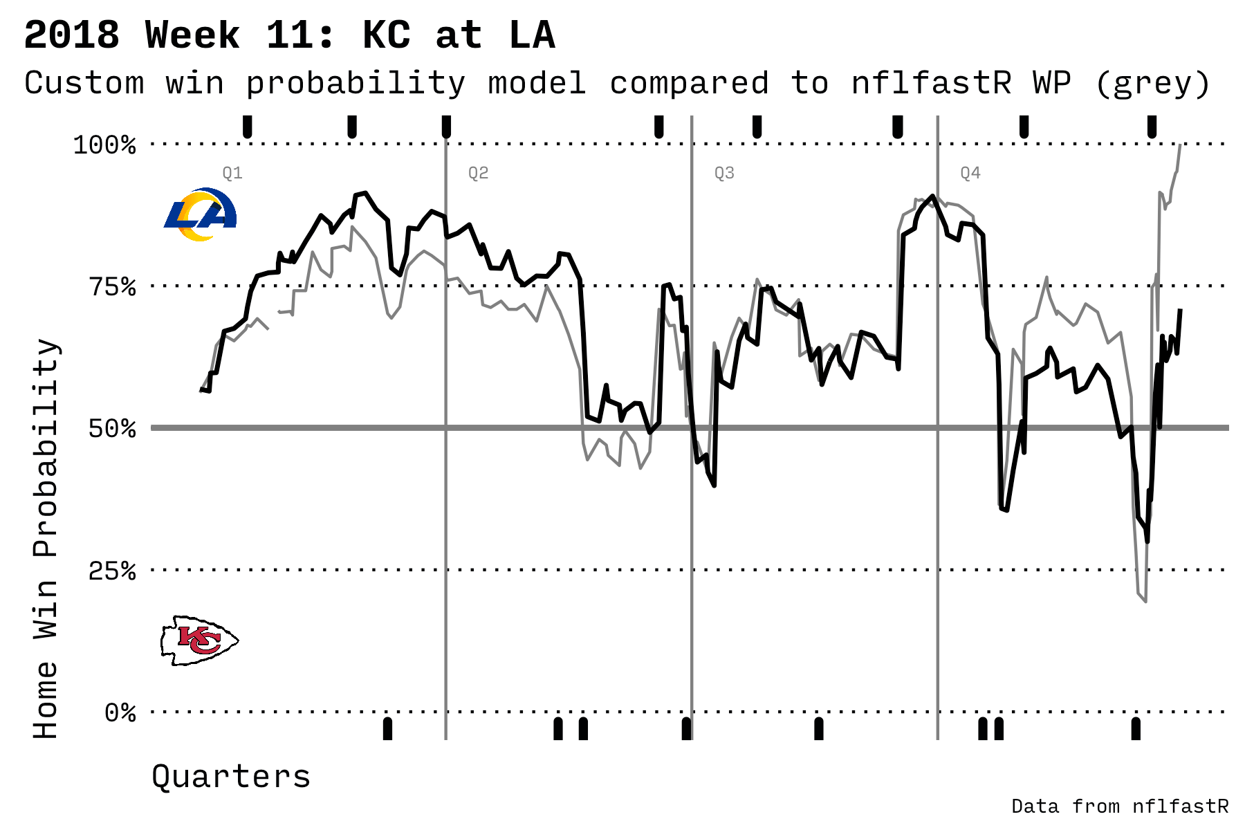
One of the highest scoring and most exciting Monday Night Football games
R Techniques
While coding up the model I stumbled onto a few features of R that I’ll certainly use in the future.
Build a function for logic statements
R provides basic flow control functions like ifelse as well as and/or syntax with && or ||. But it’s better to use the single character & and | for speed and for processing an entire vector. Speed is important since the dataset includes over 400,000 individual plays and could grow to include many more if more seasons are included.
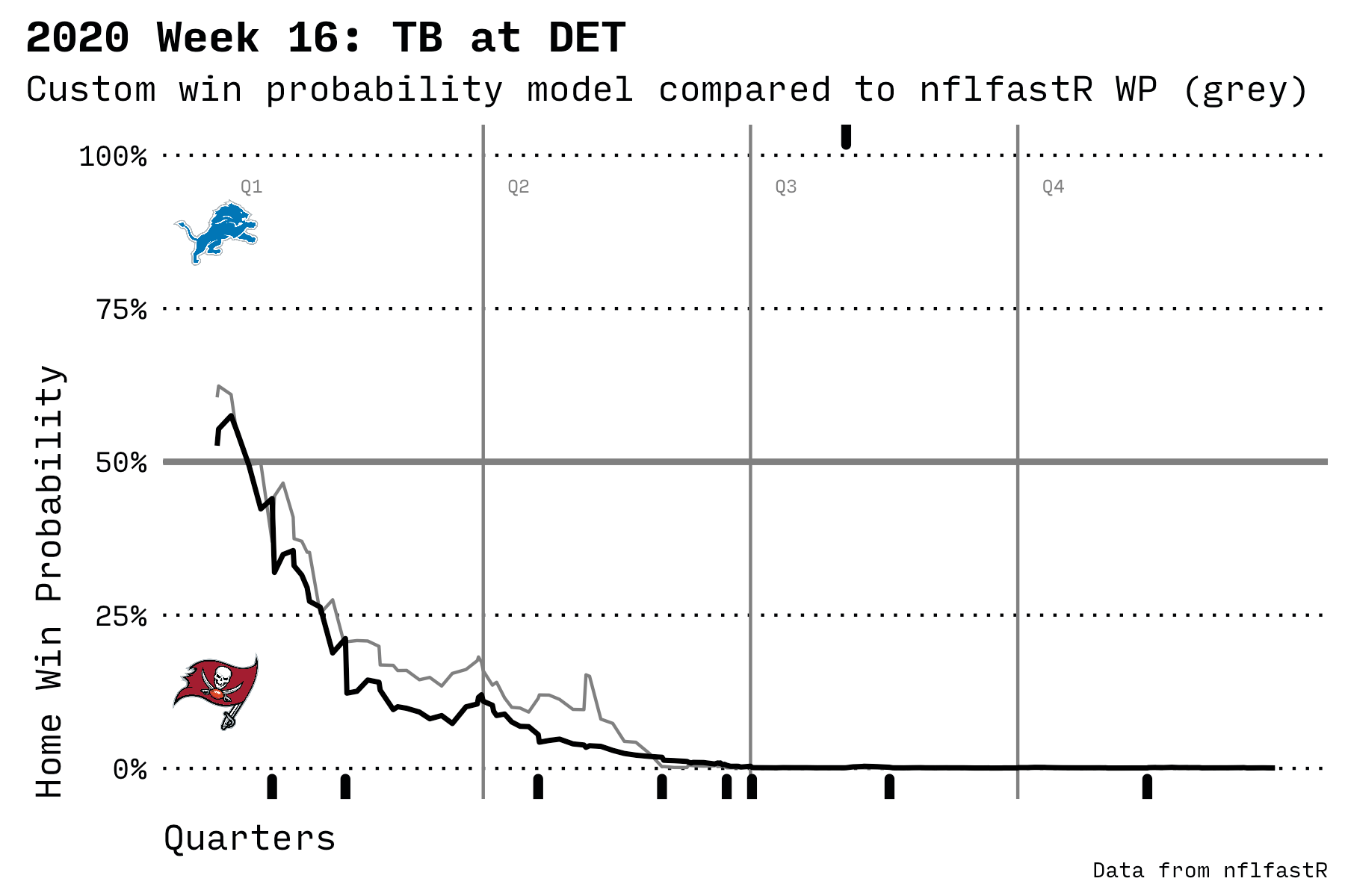
I needed a new column to draw the rug, a set of marks that indicate a scoring play for the home or away team. Based on the columns provided by nflfastR, what constitutes a scoring play?

The rug is the set of marks that indicate a scoring play by the home or away team
The logic for building the home_scoring_play column must examine six other columns to indicate a scoring play when:
- The current team scores a touchdown
- OR the current team scores an extra point or a field goal
- OR the other team possesses the ball and there is a safety (i.e. the defense scored)
The best way to do this in a readable way is to write a function that describes the complex conditional with & and | and then return the result. That function can be called by mutate or other data munging functions in order to quickly process an entire vector. Here’s the function.
is_scoring_team <-
  function(posteam,
           play_type,
           td_team,
           safety,
           this_team,
           that_team) {
    (td_team == this_team) |
      (posteam == this_team &
         (play_type == "extra_point" |
            play_type == "field_goal")) |
    (posteam == that_team & safety == 1)
  }
Then call with:
pbp_data %>% mutate(
  home_scoring_play = is_scoring_team(posteam,
                                      play_type,
                                      td_team,
                                      safety,
                                      home_team,
                                      away_team)
)
I think that conditional functions will clean up some other code I’m using in other projects.
Write a function that operates on rows
In other cases I couldn’t find a way to process an entire vector, so I needed to use the if statement or str_interp or other functions that need to be handed a single row at a time.
It turns out that this is possible by using the apply function. The 1 argument tells it to send the logos dataset to the cache_logo_image function one row at a time.
logos %>%
    mutate(team_logo_local = apply(logos, 1, cache_logo_image))
Then I can access column values from the single row with matrix-style double brackets (such as logo[['team_abbr']] below).
# Be nice to the ESPN CDN by storing team logo images locally.
cache_logo_image <- function(logo) {
  local_filename = str_interp("data/${logo[['team_abbr']]}.png")
  if (!file.exists(local_filename)) {
    download.file(logo[['team_logo_espn']], local_filename)
  }
  return(local_filename)
}
Not only is this good internet behavior, it also speeds up my program because I can read team logos from a local directory instead of downloading them remotely every time.
Conclusion
This was a fun project and mostly transpired over the December holidays. Next, I think I’d like to try other kinds of machine learning, neural networks, TensorFlow, or other tools to build similar predictive models.
- Code for this project on GitHub
- My linear regression model post
- My high contrast theme
- A Medium post using nflscrapr to build a win prediction model
- The nflfastR package
- nflfastR field descriptions
- The nflfastR WP model description
- The glm function
- The xgboost package
Design Notes
This post uses a half dozen components that I designed over the last year (the inline sidebar, the wide and dark alternate section), plus a few more (such as the triad of numbers at the top).
I used CSS Grid for parts of the layout, which is enjoyable to use and has significantly reduced my frustration with CSS layouts.


